Observational Distribution Benchmark (Layer 1)

What is Observational Data?

Observational data refers to any data that is passively collected, without any specific interventions performed. The name observational comes from the fact that the data collector is just observing the real world, without acting in it. This type of data reflects natural patterns in the world, and the vast majority of data we encounter is observational. This includes various forms of data such as surveys, administrative records, public health records, electronic health records, company records and so on.

An illustrative example for distinguishing observational from non-observational data may be helpful here. For instance, consider the investigation of tutoring and exam performance. Students who attend private tutoring often perform better on tests — but this conclusion is drawn from observational data, in which the choice of tutoring follows its natural regime. In this natural regime, families choosing tutoring may differ in other ways, such as socioeconomic status (SES). Therefore, it may co-occur that tutoring and high exam performance are both caused by better SES, which allows the parents to spend more time helping their kids study. In this context, it would be possible to obtain different kind of data, coming from a randomized controlled trial (RCT). In the RCT setting, we would randomly assign tutoring to different students, and then check whether the correlation of tutoring with improved exam performance still exists. This type of data is referred to as interventional, since we actively changed the way in which tutoring is assigned (in our case, at random). As a consequence of randomization, tutoring choice may no longer be correlated with the family's SES, in this way avoiding possible spurious correlations. Observational data, by contrast, reflects natural patterns without intervention, and may reflect both causal and spurious correlations. You can read more about observational and interventional data in the section on Pearl’s causal hierarchy.

How Can Models Exhibit Knowledge of Observational Distributions?

We will label observational distributions in the real world with \( P(V) \), where \( V \) is the set of variables we are studying. As a running example for illustrating our benchmark, we will be interested in smoking rates across age groups. This information is encoded in the distribution \(P(V_X, V_Y)\), where \( V_X \) denotes age, and \(V_Y\) denotes smoking. To obtain the distribution of age and smoking in the real world, we refer to National Survey on Drug Use and Health (NSDUH) 2023, collected by the Substance Abuse and Mental Health Services Administration (SAMHSA). The NSDUH provides information on substance use and mental health in the US, and includes information about cigarette usage across demographics.

Example: NSDUH – Smoking by Age (Question-Answer Prompting)

Let \( V_Y \) be whether a person has ever smoked, and \( V_X \) their age. From the NSDUH dataset, we can recover the true distribution \(P(V_Y \mid V_X)\). Our goal is to compare this distribution to the models distribution \( \tilde P(V_Y \mid V_X) \). The model's distribution is elicited using the following type of question. For the age \( v_X = 16 \) years, we ask the model the following question: "Has a person aged 16 ever smoked a cigarette?"

The model is offered to choose between answers {"yes", "no"}, where the answers are labeled with letters of the alphabet:

A. yes 
B. no

After asking such a question to a model, we inspect the relative probabilities for answers "A" and "B", and from this compute the proportion of individuals for whom the model believes are smokers. For instance, if the answer "A" has a probability of 1%, and answer "B" of 3%, the relative probability a positive answer is 0.01 / (0.01 + 0.03), and we infer that \( \tilde P(V_Y = 1 \mid V_X = 16) = 25 \% \). Analogous questions are asked for all other values of \(v_X\).

The above example illustrates several important concepts appearing in the benchmark. First, it illustrates the concept of a task, in this case the task of recovering smoking status across age. The task is defined by the pair \(V_Y\) (outcome variable of interest; in this case smoking) and the conditioning variables \(V_X\) (in this case age). The goal in the task is to recover the distribution \(P(V_Y \mid V_X)\), for which different LLMs can be used. However, in the task, we want to compare the distribution inferred by the LLM with the ground-truth. This brings us to the second important concept of reference dataset, a ground-truth data source from which the true distribution can \(P(V_Y \mid V_X)\) can be determined. In our example, this is the NSDUH dataset from SAMHSA, which records smoking status of different individuals, and provides sample weights to make the dataset representative at the national level. Finally, the third key concept is the prompting technique. In the above example, we used the so-called question-answer prompting technique. The model is asked a question, while the model's probabilities are extracted from its next-token prediction probabilities over the possible answers. There is also an alternative way for eliciting model probabilities, described in the next example:

Example (Continued): NSDUH – Smoking by Age (Likelihood Prompting)

The alternative way to elicit the model's distribution is to ask the following: "What is the probability that a person aged 16 ever smoked a cigarette?". The model is offered to choose between probability levels, where the answers are labeled with letters of the alphabet:

A. 0% 
B. 0-5% 
C. 5-10% 
... 
U. 95-100% 
V. 100%

After asking such a question to a model, we inspect which of the answers "A" to "V" has the highest next-token probability. For instance, if the answer "A" has the highest probability, we set \( \tilde P(V_Y = 1 \mid V_X = 16) = 0 \% \), whereas if the most likely answer is "B" we set \( \tilde P(V_Y = 1 \mid V_X = 16) = 2.5 \% \) as the midpoint of the interval 0-5%, and so on. By repeating the above type of question for different ages \(v_X\), we have an alternative way of eliciting the model's distribution.

The above way of eliciting the model distribution is called likelihood prompting. We investigate both the question-answer and likelihood prompting in our benchmark.

Distribution at Age 16

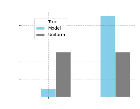
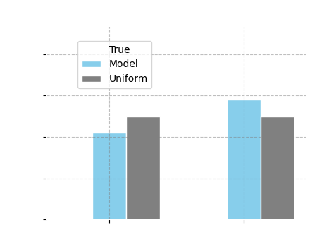
After performing the above question-answering exercise, we can visualize the ground-truth smoking distribution for age 16, together with the distribution inferred from the model. In addition, we also plot the uniform distribution, which chooses between answers at random, assigning each answer equal probability (in this case, both answers "yes" and "no" are given a 50% probability). This distribution represents answers without having any idea about the true probabilities.

Figure A: Aligned model distribution.

Figure B: Misaligned model distribution.

The above plots illustrate two settings: for Model A (in Figure A, left), we see an LLM distribution exhibiting partial knowledge about the observational distribution. The model's distribution does not align perfectly with the truth, but it's much closer to the ground truth than the uniform distribution. For Model B (in Figure B, right), however, the model distribution is much further from the ground truth, overestimating significantly the proportion of individuals who ever smoked a cigarette. These plots raise a natural question: how do we assign a score to a model, determining how well it approximates reality? This is described in detail below.

Comparison Plot

The above question-answering exercise can be repeated for different age groups, and we may compare the true probabilities with the model's probabilities across a range of ages.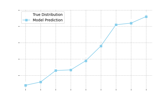

How Do We Score Model Answers?

To evaluate how well a model understands observational patterns, we compare the model's predicted distribution \( \tilde{P}(V_Y \mid V_X) \) to the true distribution \( P(V_Y \mid V_X) \) from the dataset. The core idea is simple: if the model's distribution closely matches the actual population distribution, it receives a high score (maximal score is 100). If the model's predictions are far off — for example, if it guesses randomly or gives constant answers regardless of the context — it receives a low score (minimal score is 0).

Technically, we use a distance metric called the \( L_1 \)-norm to quantify the difference between distributions. This metric just sums up how much the model's predicted probabilities differ from the real ones. However, instead of reporting raw distances, we turn them into a score S from 0 to 100, where S = 0 and S = 100 are defined as follows:

S = 100 means the language model's answers are statistically indistinguishable from the true distribution - after accounting for sampling variability in the survey data such as NSDUH.
S = 0 means the model does not do better than guessing uniformly at random.

Finally, the model's score is linearly interpolated between the poor (S = 0) and perfect answers (S = 100). This gives us a flexible scale that reflects how close the model's knowledge is to the empirical truth, and such a scoring strategy can be used across different tasks (beyond smoking status across age groups).

Which Tasks Do We Study More Broadly?

Our benchmark spans a diverse set of U.S. population datasets, each offering a unique lens into social, economic, health, and behavioral patterns. Below we a list of the datasets studied, along with the specific statistics we investigate. We emphasize that the list is not exhaustive, but rather represents an initial first step towards a systematic study of observational distributions. We expect that numerous other datasets will be added to the benchmark in the future, including data from other countries.

American Community Survey (ACS) 2023: Conducted by the U.S. Census Bureau, the ACS collects detailed demographic, social, economic, and housing data annually. We focus on income, education, and employment across different demographic groups.
National Health and Nutrition Examination Survey (NHANES) 2021–2023: Administered by the CDC, NHANES combines interviews and physical exams to assess health and nutrition in the U.S. population. We analyze obesity, diabetes, and dietary habits by demographics.
Behavioral Risk Factor Surveillance System (BRFSS) 2023: A CDC-run telephone survey system that tracks health-related behaviors and conditions. We examine exercise habits, diabetes, blood pressure, asthma, cholesterol, and impairments across U.S. states.
Medical Expenditure Panel Survey (MEPS) 2023: Conducted by the AHRQ, MEPS collects data on health service usage, expenditures, and insurance. We study patterns of healthcare spending, utilization, and coverage across groups.
National Survey on Drug Use and Health (NSDUH) 2023: Collected by SAMHSA, NSDUH provides data on substance use and mental health. We explore alcohol, cigarette, marijuana, cocaine, and heroin use across demographics.
Survey of Consumer Finances (SCF) 2022: Sponsored by the Federal Reserve Board, the SCF details U.S. household finances. We investigate food spending, home ownership, assets, and debt by demographic characteristics.
General Social Survey (GSS) 2022: Conducted by NORC at the University of Chicago, the GSS captures U.S. adults’ social attitudes, behaviors, and demographics. We analyze political views and party affiliation across age, sex, race, education, and income.
Integrated Postsecondary Education Data System (IPEDS): Maintained by the U.S. Department of Education, IPEDS collects institutional-level data. We study degree attainment by sex across college programs.
Bureau of Labor Statistics (BLS) 2023: The U.S. Department of Labor provides data on occupations and worker demographics. We examine occupational distributions by sex and race.
FBI Arrest Statistics (UCR Program): Compiled by the FBI’s Uniform Crime Reporting Program, this dataset records arrest statistics nationwide. We explore crime rates by race and sex.

The performance of different language models on our benchmark can be found at this page, whereas the full list of tasks, with model scores, is found here.